Medical Foundations 1
Chapter 2Primer on Evidence-Based Practice in Clinical Skills
Introduction
Throughout medical school, you will learn different Evidence-Based Practice skills as an important epistemological way of knowing. In Clinical Skills, we focus particularly on Clinical Decision-Making Models (Part 1) and Evidence-Based Diagnosis (Part 2). As you learn different screening questions and physical exams, it is helpful to know the evidence behind these tests e.g. how much does performing this physical exam test help me answer a clinical question? Where pertinent, Sensitivity, Specificity, or Likelihood Ratios are included in the Why Check for a given physical exam test. At the end of each Chapter, tables of Evidence-Based Clinical Questions are presented (including Why Check values). This Primer is intended to help make sense of this terminology. Additional information on Therapy Studies (Part 3), Critical Appraisal (Part 4), the Hierarchy of Evidence (Part 5), and Measures of Population/Community Health (Part 6) are included for your reference. For further information you are encouraged to visit the AFMC Primer on Population Health (https://phprimer.afmc.ca/en/).
Part 1: Clinical Decision-Making Models in Practice
The following model was developed by Dr. Alba DiCenso from the McMaster School of Nursing and is introduced in the Professional Competencies curriculum. It outlines 4 components that must be considered in making clinical decisions with patients, mediated by clinical expertise, as follows:
- Clinical State, Setting, Circumstances: Includes clinical skills (e.g. History, Physical Exam)
- Research Evidence: Including evidence-based practice skills (e.g. in weighing the evidence for different management options)
- Key Idea: Evidence by itself does not tell us what to do
- Key Idea: Know the evidence behind your decisions; when multiple paths acceptable based on available evidence, share this info.
- Health Care Resources: Understand resource availability, allocation.
- Patient Values, Preferences and Actions: Including patient-centred communication skills and narrative competencies.
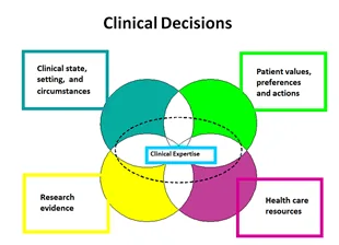
In terms of roles in decision-making, 4 general models are outlined:
| Approaches | Parental | Clinician as Perfect Agent | Informed Choice | Shared Decision Making |
|---|---|---|---|---|
| Information Flow about OPTIONS | Clinician ↓ Patient | Clinician ↓ Patient | Clinician ↓ Patient | Clinician ↑↓ Patient |
| Information Flow about VALUES and PREFERENCES | Clinician ↓ Patient | Clinician ↑ Patient | Clinician ↑ Patient | Clinician ↑↓ Patient |
| Deliberating and Deciding | Clinician | Clinician | Patient | Clinician & Patient |
Part 2: Evidence-Based Diagnosis – Understanding, applying evidence for specific tests (e.g. physical exam tests)
Important Definitions
| Truth: Positive | Truth: Negative | |
|---|---|---|
| Test Result: Positive | A | B |
| Test Result: Negative | C | D |
- Sensitivity (A / (A+C)): The True Positive Rate – Proportion of patients with disease who have a positive test
- Clinical Relevance – SnNOUT: Sensitive Tests when negative are useful to rule out disease
- Specificity (D / (B+D)): The True Negative Rate – Proportion of patients without disease who have a negative test
- Clinical Relevance – SpPIN: Specific Tests when positive are useful to rule in disease
- Positive Likelihood Ratio (LR+ve) (Sensitivity / (1−Specificity)): Probability a positive test would be expected in a patient with disease compared to likelihood a positive test would be expected in a patient without disease.
- Clinical Relevance: LR +ve quickly communicates how much a given positive test changes the probability of a given diagnosis. Tables comparing Likelihood Ratios help compare which tests have the greatest diagnostic value.
- Details: LR >1 ↑ probability of disease, LR from 0-1 ↓ probability of disease. LR = 1 does not change probability of disease (i.e. not helpful).
- Note: Check 95% Confidence Interval – if this crosses 1 (e.g. 95% confidence interval from 0.5-3), the test’s utility in answering that specific clinical question is not high.
- Negative Likelihood Ratio (LR-ve) ((1−Sensitivity) / Specificity): Probability a negative test would be expected in a patient without disease compared to likelihood a negative test would be expected in a patient with disease.
- Clinical Relevance: LR -ve quickly communicates how much a given negative test changes the probability of a given diagnosis. Tables comparing Likelihood Ratios help compare which tests have the greatest diagnostic value.
Clinical Relevance: Converting from Pre-Test to Post-Test Probability Using Likelihood Ratios and Nomograms
- Key Idea: Your history, exam and investigations should help rule in or rule out items on the Differential Diagnosis (DDx).
- Pre-Test Probability: Before your physical exam test, given clinical picture thus far, what is the probability your patient has the disease? Disease prevalence, patient risk factors and exposures identified on history can influence pre-test probability.
- Post-Test Probability: After your physical exam test, what probability would you assign the patient has the given disease?
- Method 1 – Use of Nomograms: Using a Nomogram (see example below), with a point on Pre-Test probability and on Likelihood Ratio columns, draw a line through these to the Post-Test probability column. This is your post-test probability.
- Method 2 – Calculate Post-Test Probability:
- (1) Pre-Test Probability (x, as a decimal) → Pre-Test Odds = x / (1−x)
- (2) Pre-Test Odds (y) x Likelihood Ratio (LR) = Post-Test Odds (z) → Note: You can multiply Likelihood Ratios together – where each likelihood ratio must be due to independent pathophysiology in order to be readily multiplied
- (3) Post-Test Odds (z) → Post-Test Probability = z / (1+z)
- Method 3 – Simplified Approximation Method to Apply Likelihood Ratios1: For pre-test probabilities between 10 and 90% (outside of this, this simplified method is not valid), an approximate change in probability is shown (see right – actual equation: ∆probability ≈ 0.19 × log LR). In the guide, the colour code shown is applied to tables of Likelihood Ratios, where confidence interval (CI) does not cross 1 – if it does, cell is grayed out as a non-helpful test
| LR | Approx. Change in Probability |
|---|---|
| 0.1 | -45% (LR ≤ 0.1 in guide) |
| 0.2 | -30% (0.5 > LR > 0.1 in guide) |
| 0.5 | -15% (1 > LR ≥ 0.5 in guide) |
| 1 | 0 (95% CI range crosses 1 in guide) |
| 2 | 15% (1 < LR ≤ 5 in guide) |
| 5 | 30% (5 < LR < 10 in guide) |
| 10 | 45% (LR ≥ 10 in guide) |
Worked Example
You see a patient in clinic with new shortness of breath. After gathering a history, you estimate a pre-test probability of 40% this patient has pneumonia. Your collect the following vital signs: Temp 38.2C, RR 30, HR 90, BP 120/80, O2sat 95% on Room Air**.** Referring to Resp Exam Clinical Question 1 – Does this Patient Have Pneumonia, you identify Likelihood ratios for each of vital sign (see above – highlighted in yellow which ones apply to our patient, a combination of positive and negative findings). You calculate Post-Test probability after collecting these vitals, before you proceed with your physical exam, trying each of these 3 methods.
| Finding | LR+ve (95% CI) | LR-ve (95%CI) |
|---|---|---|
| Temp >37.8C | 2.0 (1.5-2.6) (about +15%) | 0.7 (0.6-0.8) (about −15%) |
| RR >28/min | 2.0 (1.4-2.8) (about +15%) | 0.8 (0.7-0.9) (about −15%) |
| HR >100 beats/min | 1.6 (1.4-1.7) (about +15%) | 0.8 (0.7-0.9) (about −15%) |
Method 1 – Nomogram: You use the Nomogram for each likelihood ratio and find the Post-Test probability to be about 70%.
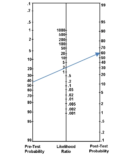
Test 1 Post-Test Probability – LR+ve 2.0
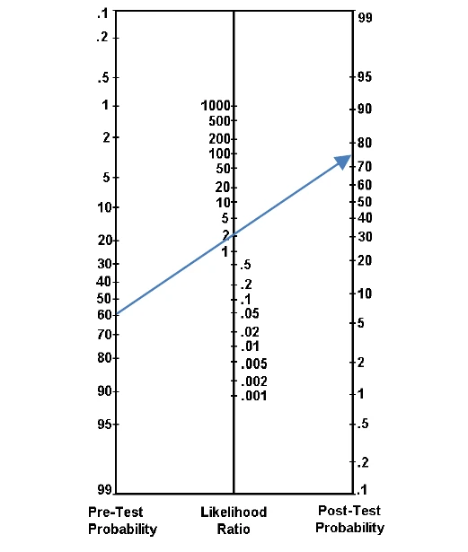
Test 2 Post-Test Probability – LR+ve 2.0
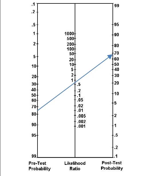
Test 3 Post-Test Probability – LR-ve 0.8
Method 2 – Calculation: To calculate a more exact Post-Test probability, you do a formal calculation as follows:
| Pre-Test Probability | Pre-Test Odds | Post-Test Odds | Post-Test Probability |
|---|---|---|---|
| 0.40 | 0.40 / (1 − 0.40) = 0.66 | 0.66 × 2.0 × 2.0 × 0.8 = 2.112 | 2.112 / (1 + 2.112) = 0.68 |
Method 3 – Simplified Approximation Method: As pre-test probability is between 10-90%, we can use an approximation method. Given pre-test probability of 45%, our two tests with LR+ve of 2.0 raise the post-test probability by (15% x 2 = 30%) to 70%. Our LR-ve of 0.8 will lower this slightly (0.19 x log(0.8) =0.018, or about 2%) to give a post-test probability of 68%.
Conclusion: Using each method, your pre-test probability this patient has a pneumonia before completing a focused physical exam has risen from 40% to 68% after reviewing the patient’s vital signs and pertinent Likelihood Ratios.
Other Relevant Diagnostic Test Properties
| Truth: Positive | Truth: Negative | |
|---|---|---|
| Test Result: Positive | A | B |
| Test Result: Negative | C | D |
- Prevalence ((A+C) / (B+D)): Burden of disease – ratio of patients who have the disease to patients who do not have the disease in a given population – Prevalence only applies to patients matching population under study with same baseline risk (i.e. Ask: Do these results apply to my patient?)
- Positive Predictive Value (PPV) (A / (A+B)): Proportion of patients who have a positive test result who do have the disease in a given population – PPV only applies to patients matching population under study with same baseline risk
- Negative Predictive Value (NPV) (D / (C+D)): Proportion of patients who have a negative test result that do not have the disease in a given population – NPV only applies to patients matching population under study with same baseline risk
- Kappa (κ): Measure of reliability of Inter-observer agreement i.e. how often multiple clinicians examining a patient would agree about presence or absence of a particular physical exam finding beyond random chance.
- Details: κ range from -1 to 1; if κ <0, agreement worse vs. random chance; if κ 0-0.2 = Slight agreement; κ 0.2-0.4 = Fair; κ 0.4-0.6 = Moderate; κ 0.6-0.8 = Substantial; κ 0.8-1.0 = Perfect agreement; if κ > 0.8, the test is considered Excellent
- Clinical Relevance: If κ is low, this can undermine findings and limit ability to apply a physical exam test confidently.
Part 3: Key Definitions for Therapy Studies
- Experimental Event Rate (EER): How much an event occurred in the Treatment Group
- Control Event Rate (CER): How much an event occurred in the Control Group (e.g. Placebo group; may approximate baseline risk if non-specific to conditions of the study)
- Clinical Relevance: Ask before applying study clinically – Does CER make sense as baseline risk for my patient population?
- Absolute Risk Reduction (ARR = CER − EER): What percent event reduction occurred in Treatment vs. Control group?
- Clinical Relevance: ARR is Prevalence Dependent – As CER ↑, this means ARR ↑ as well
- Relative Risk Reduction (RRR = (CER−EER) / CER = ARR / CER): How much less likely is event in Treatment vs. Control group?
- Clinical Relevance: May be misleading as it depends on 1/CER (e.g. if baseline risk rare, a small ARR may create large RRR)
- Number Needed to Treat (NNT = 1 / ARR = 1 / (CER−EER)): How many patients would need to be treated for 1 to receive a benefit?
- Clinical Relevance: NNT is prevalence dependent i.e. as CER ↑, NNT ↓; NNT is also time-dependent – where we need to be mindful when comparing 2 NNT values with different time frames reported.
- Key Idea: The persuasiveness of sharing statistics to patients when exploring potential treatment options depends both on the patient’s understanding of the number itself, and their perception of the implied size and effect.
- What Does the Evidence Show? RRR is most persuasive statistic; ARR and NNT equally persuasive, but less so than RRR.
Part 4: Critical Appraisal “How Can We Establish Whether Presented Evidence is Trustworthy?”
- GRADE Approach: International grading system - Grades of Recommendation, Assessment, Development and Evaluation – providing a framework to inform how confident you can be in a given guideline
- PICO Format: Framing a clinical question to do a proper literature search: Patient, Intervention, Comparator, and Outcome.
- To do a meta-analysis, the data sets being pooled must share a common PICO format
- Systematic Review: Aim is to find all of the applicable best evidence to answer your PICO-formatted question.
- The report you generate answers the state of research on THIS PICO QUESTION at THIS TIME.
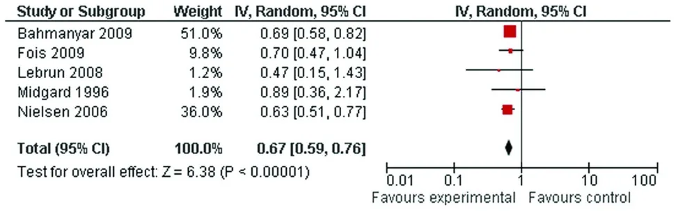
- Forest Plot: Helps you to decide whether what you are reading is worthwhile or not in medical decision making
- Inconsistent Forest Plot Picture: Means in each study are highly dispersed
- Consistent Forest Plot Picture: Means in each study within confidence intervals of one another
- Note: One benefit of pooled data sets is to ↓ Confidence Interval (i.e. more precise summary estimate of effect)
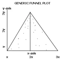
- Funnel Plot: Used to check for existence of PUBLICATION BIAS. On X axis is the measured effect of the study, while on the Y axis is the size of the study. A study without publication bias should have the largest studies near the apex of the triangle plotted around average estimate of the effect, while smaller studies will be clustered evenly about both sides of the average.
Assessing Confidence
High Confidence
- Able to Make a Strong Recommendation: Benefits & Risks/Costs CLEARLY IMBALANCED
Starting Point
- RCT: Begins with HIGH Confidence
- Observational Study: Begins with LOW Confidence
Parameters that ↓ Confidence
- Risk of Bias (e.g. Lack of blinding; Loss of patients to follow-up)
- Inconsistency between studies (e.g. Some recommend for treatment, others recommend against it)
- Indirectness (e.g. not applicable to your patient)
- Imprecision (e.g. Wide confidence intervals)
- Publication Bias: Tendency for an overestimate of the effect since positive studies are about 3X more likely to be published than negative studies. You can tell this based on the shape of a FUNNEL PLOT
Parameters that ↑ Confidence
- Large magnitude of study; Common inclusion criteria for study
- Dose Response Curve – re Evidence of a Gradient Effect
How Can We Trust Causal Relationships Presented?
- Strength of association of outcome with exposure; Consistency with other investigations
- Time sequence re accounting for potential exposures prior to study
- Dose-Response Relationship demonstrated with the exposure
- Biological Credibility: Is it possible to make a sensible model? Note: Serendipity tends to precede mechanism elucidation
Part 5: Study Design – Hierarchy of Evidence & Key Terms
Important Definitions for Study Design
- Exposure: Differential experiences/events in groups vs. Outcomes: Death, disease, quality of life, etc.
- Prospective: Observations concurrent with study vs. Retrospective: Observations occurring after the study
- Observational: Describing an ongoing situation vs. Experimental: Measuring effect of an intervention (manipulative)
- Control: Comparison group (e.g. Placebo)
- Allocation/Randomization: How exposure is assigned (process)
- Confounding Variable: Caused by a third factor associated with both the exposure and the control group
- Bias: A systematic error in design, conduct or analysis of study resulting in mistaken estimate of exposure’s effect on the risk of disease e.g. Selection Bias; Misclassification Bias; Recall Bias; Wish Bias
Hierarchy of Scientific Evidence informing Medical Decision Making
- Systematic Reviews & Meta-Analyses
- Randomized Control Trials (RCT, Double-Blind) -Experimental study with random allocation to groups – not always possible due to ethical considerations, costs, impossibility to manipulate exposures, or rarity of the outcome under study.
- Cohort Studies – Observational study with sampling based on common exposure, followed over time (longitudinal study)
- Case Control Studies – Observational study with sampling based on groups with different outcomes, comparing groups based on reviewing exposures.
- Cross-Sectional Studies – data from a population at one specific point in time
- Case Series – tracking data of one group with known exposure
- Animal Research and In Vitro (test tube) Research
- Case Reports; Opinion Papers, Editorials
Part 6: Measures of Population or Community Health: Health as a resource for everyday life
How Do We Measure the Health of a Population or Community?
- Population or Community: Groups of people with something in common (e.g. stage of disease, shared social determinants)
- Ratio: x/y or x:y → these can be unrelated, using different units
- Proportion: A special type of ratio, where x is a subset of y (x/y) using same units
- Rate: Incorporating an element of time
- Incidence: # of new events in period / # of persons exposed to risk in period → Proportion, NOT A RATE
- Prevalence (Point Prevalence): # existing in period (+ incidence) / # persons at risk → Proportion, NOT A RATE
- Attack Rate (AR, Infectious Diseases): Incidence cases of diseases / total exposed → Proportion, NOT A RATE
- Relative Risk (RR, Risk Ratio): Risk of disease among exposed / Risk of disease among unexposed (comparing the AR)
- Standardization: Used to enable comparing of different populations. In order to make meaningful comparisons, need to make both populations either apples or oranges (control for confounding variables)
- Direct: Your rate, other population’s weight (to standardize and allow comparison)
- Indirect: Other population’s rate, your populations weight (e.g. age structure, other confounding variables)
- AFTER STANDARDIZATION: Get a Standard Mortality Rate (SMR) for each of the populations, facilitating a comparison between the two (re what is expected)
References
-
McGee S. Simplifying likelihood ratios. J Gen Intern Med. 2002;17(8):647-650. ↩